Cross Stream
AI
Home
About
Examples
Contact
Latest Articles
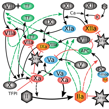
The Coagulation Cascade: Information Geometry in your blood, stream-lined
Understanding AIDS treatment
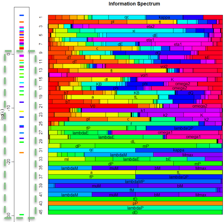
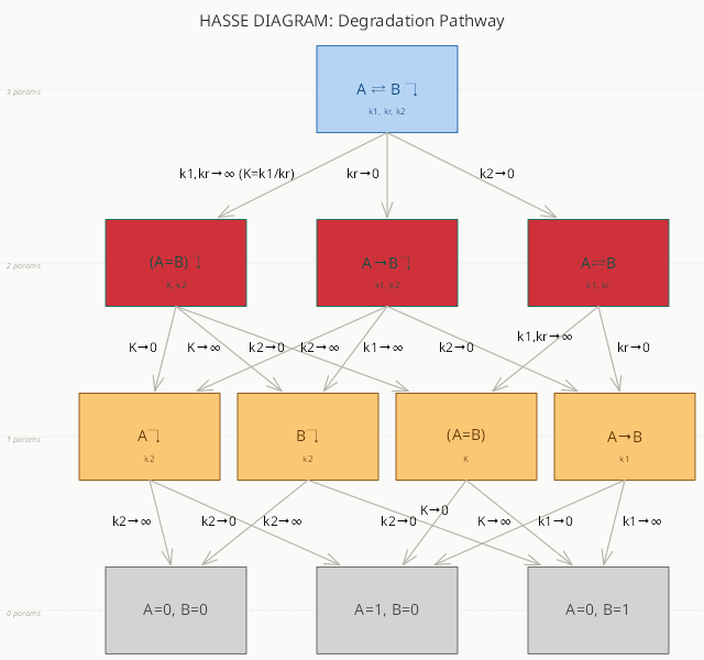
Information Geometry 101