Information Geometry 101

When we talk about models, whether they describe molecules in a cell, financial markets, or climate systems, it's easy to get lost in equations and parameters. Information geometry offers a different lens: it treats families of models as geometric objects, with shapes, distances, and directions that capture how models relate to one another. That means we can ask questions like "Which models are nearly indistinguishable?" or "Which parameters really matter?" in a precise yet intuitive way. The beauty is that once you see models as living on a continuum from complex to simple (but physically interpretable at any level of complexity), a whole toolkit of geometric reasoning becomes available. We can then understand our system at a profound level, while comparing and predicting models with far more clarity than brute force alone.

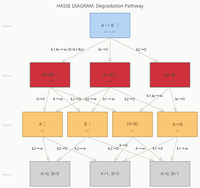
The A ⇌ B ↴ model

Consider a simple degradation pathway in which a precursor molecule A converts reversibly to an intermediate B, which is then irreversibly cleared from the system:

$$\dot{A} = -k_1 A + k_r B$$ $$\dot{B} = k_1 A - k_r B - k_2 B$$

with initial conditions A(0) = 1, B(0) = 0. The three parameters are the forward conversion rate k₁, the reverse rate k_r, and the clearance rate k₂. This could describe a drug and its active metabolite, a signaling protein held in a reversible inactive form, or any two-pool system where the second pool drains. The mathematics doesn’t care which story you prefer.

Reducing from three parameters to two

The key first step is to ask: which single-parameter reductions are legal? “Legal” here has a precise meaning — the reduced model must still be identifiable from data, meaning all remaining parameters can in principle be estimated. Because A(0) = 1 and B(0) = 0, the system only ever gets going if A can actually convert to B. This makes k₁ = 0 illegal as a first step: if nothing ever leaves A, then B remains zero forever and neither k_r nor k₂ has any observable effect. You would be reducing three parameters to one in a single move, which violates the one-step rule of the Hasse diagram.

Similarly, k₂ → ∞ is illegal: instantaneous clearance of B collapses the system to a state where B ≈ 0 at all times, which makes k_r unidentifiable (there is nothing to flow back from B to A). For the same reason, k₁ → ∞ alone is illegal — sending only k₁ to infinity while holding k_r fixed causes A to drain instantly, but since nothing constrains the ratio in which it returns, you again lose identifiability.

The three legal reductions are:

k_r → 0 (model 2b): A → B ↴. The reverse flow vanishes, leaving a purely irreversible chain. Both k₁ and k₂ remain identifiable from the time courses of A and B. This is perhaps the most familiar pharmacokinetic model.

k₂ → 0 (model 2c): A ⇌ B. Clearance is negligible, and B simply accumulates in reversible equilibrium with A. The system eventually settles at a fixed ratio A/B = k_r/k₁, with both rate constants identifiable from the approach to equilibrium.

k₁, k_r → ∞ keeping K = k₁/k_r fixed (model 2a): (A=B) ↴. When both conversion rates are fast relative to clearance, A and B equilibrate almost instantaneously. The details of k₁ and k_r individually become irrelevant — only their ratio K matters, because the equilibrium fraction of B is K/(1+K). The effective clearance of the combined pool proceeds at rate k₂. This reduction has a different character from the other two: rather than deleting a flow, it fuses two compartments into one fast-equilibrating pool, replacing two parameters with one.

From two parameters to one

Each of the three 2-parameter models can be reduced further. Working through the legal moves carefully (always checking that the remaining parameters stay identifiable, and always reducing by exactly one parameter), we arrive at four 1-parameter models:

• k₂ only (model 1a): B is instantaneously degraded (k₂ → ∞), so the intermediate B form never appears. From the outside, it looks like A is being degraded directly at rate k₁.
• also k₂ only (model 1b): all of A has instantly become B (K → ∞), and B drains at rate k₂. The precursor pool is gone.
• K only (model 1c): clearance has been turned off (k₂ → 0), and the system sits in permanent fast equilibrium between A and B at ratio K.
• k₁ only (model 1d): conversion is irreversible and slow (k_r = 0, k₂ = 0), and A converts to B at rate k₁ with B accumulating.

Each 1-parameter model has exactly two legal reductions to a 0-parameter endpoint — a fixed steady state that requires no dynamics at all:

• {A=1, B=0}: nothing ever moved, or everything snapped back to A.
• {A=0, B=0}: everything converted and then drained.
• {A=0, B=1}: everything converted and none of it drained.

The geometric picture

Here is where the geometry becomes vivid. Each parameter in the full model is an axis, so the full 3-parameter model defines a solid three-dimensional region of parameter space — a polytope whose interior represents every possible combination of k₁, k_r, and k₂. The Hasse diagram is, in a precise sense, a map of the boundary structure of that polytope:

A=1, B=0 A=0, B=0 A=0, B=1

• One 3D interior — the full model, whose points are all (k₁, k_r, k₂) triples with all three parameters finite and positive.
• Three 2D faces — models 2a, 2b, and 2c. Each face is a boundary of the polytope reached by sending one parameter combination to an extreme value. Two of these faces (2b and 2c) are literal faces of the parameter cube (k_r = 0 and k₂ = 0 respectively); the third (2a) is a more unusual boundary, the fast-equilibrium manifold where k₁/k_r = K with both going to infinity. Note that model 2c has only two edges, meaning it forms a digon; models 2a and 2b have three edges and thus are triangular.
• Four 1D edges — models 1a, 1b, 1c, and 1d. Count the arrows in the diagram: each 1-parameter model is reachable from exactly two of the three 2-parameter faces, and each edge is therefore shared by exactly two faces. This is the combinatorial signature of a genuine geometric edge.
• Three 0D vertices — the three fixed steady states. Two of them ({A=1,B=0} and {A=0,B=1}) are each shared by three edges, while {A=0,B=0} is shared by only two edges and is thus the vertex of the digon pyramid.

Every path from the interior of the polytope to a vertex — traveling through a face, then an edge, then the vertex — is called a flag, and corresponds to a complete sequence of model reductions.

The practical implication is that information geometry turns model selection from a discrete search into a continuous navigation problem. A fitted set of parameters (k₁, k_r, k₂) is a point somewhere in the interior of the polytope. The Fisher Information Matrix evaluated at that point tells you the local shape of the parameter space, including which directions are stiff (small steps change predictions dramatically) and which are sloppy (you can traverse a long distance in that direction without changing anything observable). Sloppy directions point toward the nearest face. Following them takes you to a simpler model that fits your data nearly as well as the original. Reevaluating the FIM at the face and going in the sloppiest direction takes you to the nearest edge, and then the nearest corner. This is easy to visualize and, crucially, has a clean mechanistic interpretation at every step of the journey.