Understanding AIDS treatment

Despite remarkable progress in HIV care, the virus remains stubbornly prevalent. Over 38 million people worldwide are living with HIV, and while antiretrovirals (ART) have transformed the prognosis, they are expensive, lifelong, and fraught with adherence and side-effect challenges. Enter broadly neutralizing antibodies (bNAbs), engineered to target HIV's most conserved regions with potent precision. In animal studies, especially SHIV-infected macaques and humanized mice, somewhere from 45% to 77% achieved durable viral suppression after receiving bNAbs (Nishimura et al. 2019, Nel & Frater 2024). This is a hopeful sign, but crucially, that means more than half to a quarter did not respond as well. That discrepancy has scientists asking: why do bNAbs shine in some cases but fall flat in others? Understanding the reasons behind this differential effectiveness is key to turning these powerful molecules into equitable, reliable treatments. This is a task that information geometry could help illuminate by pinpointing the underlying biological mechanisms at play.

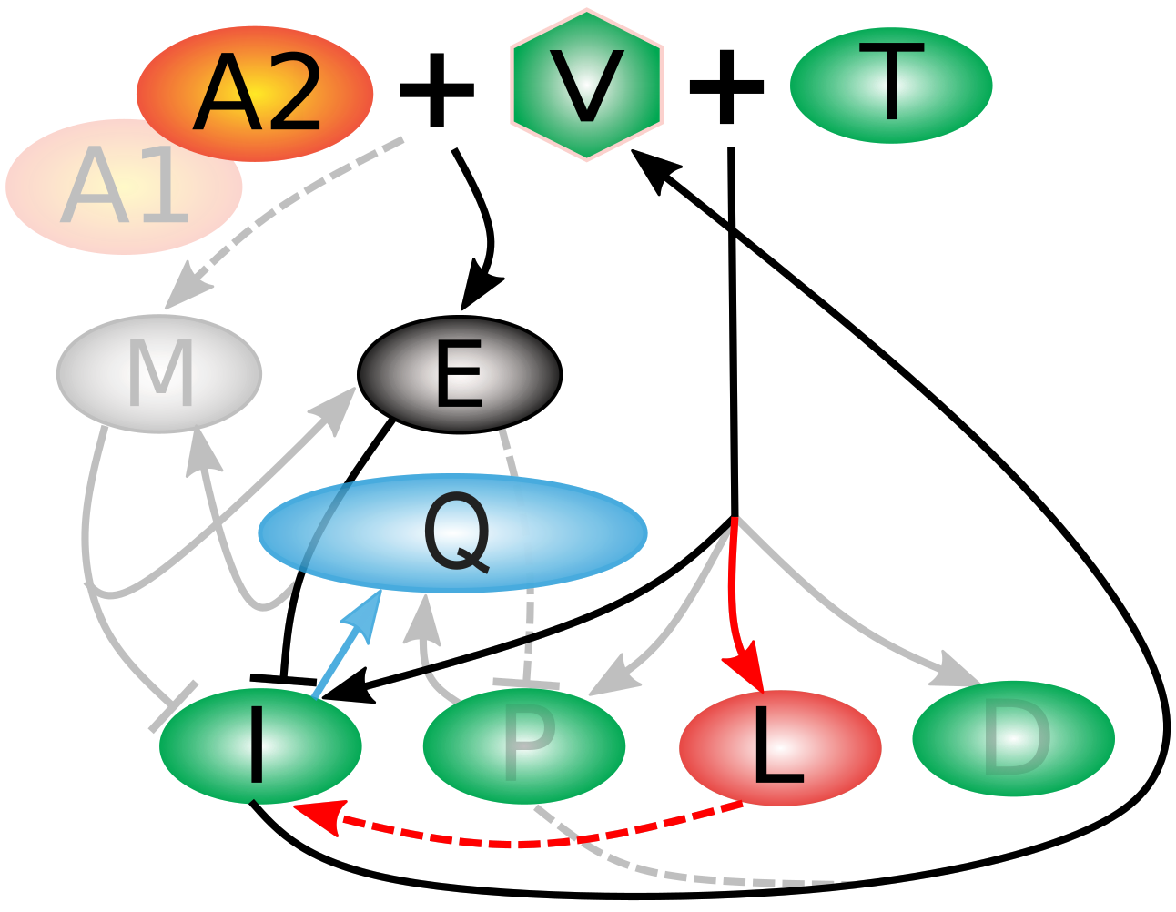
To examine this question, we built a model with 45 tunable parameters and 11 compartments by cobbling together classic models in the field (especially Desikan 2020, Funk 2001, and McLean 1994). Briefly, when a virus (V) encounters a helper T-cell (T), it creates one of four kinds of infected cells (bottom row) of which infected (I) and partially infected (P) cells produce more virus. However, when V encounters bNAb drugs A1 or A2, it activates effector cells (E) who work at efficiency Q to kill the I and P cells, and memory cells (M) to fight off later infection. Even when I and P are surpressed, latently infected cells (L) can reactivate, and some viral particles hang around in deficiently (D) infected cells.

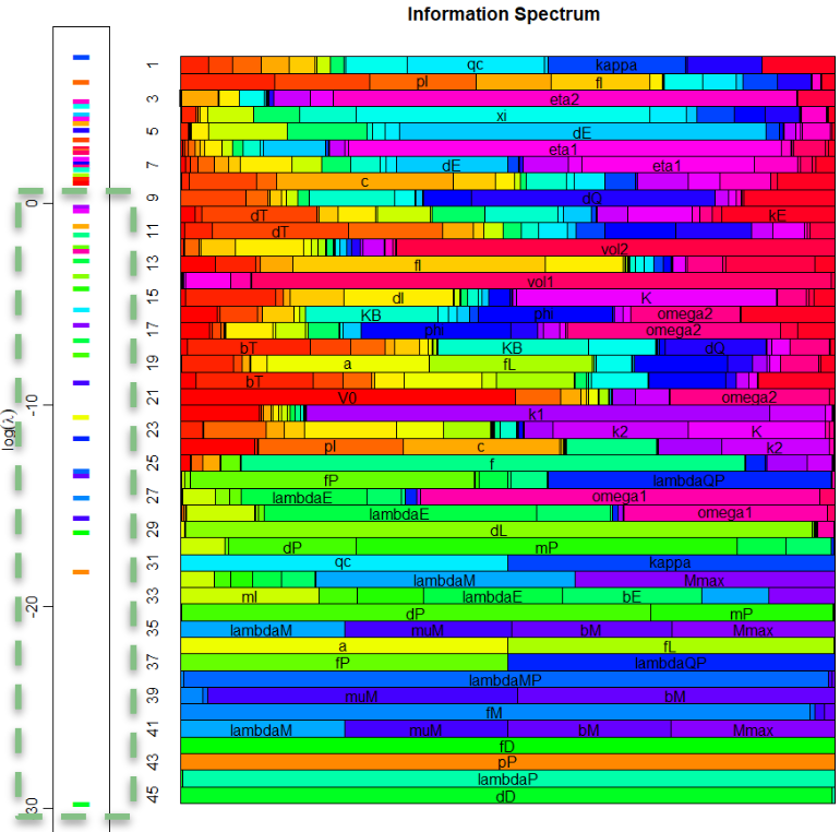
A study at the NIH (Nishimura et al. 2019, which included Anthony Fauci as one of the authors) was able to provide a great deal of data on the time course of SHIV infection in monkeys treated with bNAbs, both responders and nonresponders. We used this information to fit the model, and then evaluate the Fisher Information Matrix at that point. As you can see from the eigenvalue spectrum, there were a large number of parameters (in the red box) that could be removed from the model (the greyed-out components of the schematic above), because they were many orders of magnitude less influential on the simulated time course of infection than those parameters we kept. We determined a 22-parameter model retained the flexibility to accurately predict daily viral load for two-and-a-half years for responders, nonresponders, untreated controls, and naturally immune patients alike.

Literature Derived Model		Relevon
$$ \begin{align*} \dot{T}&=b_T-d_T T-\left(f_I+f_L+f_P+f_D\right) T V \\ \dot{V}&=p_I I+p_P P-(c+A) V \\ \dot{I}&=f_I T V-d_I I+a L-m_I E I \\ \dot{L}&=f_L T V-d_L L-a L \\ \dot{P}&=f_P T V-d_P P-m_P E P \\ \dot{D}&=f_D T V-d_D D \\ \dot{E}&=\lambda _E+\frac{\left(I+f A V+\lambda _P P\right) \left(b_E+k_E E\right)}{K_B+\left(I+f A V+\lambda _P P\right)}-\xi\frac{ Q^n E}{q_c^n+Q^n}-d_E E \\ & \qquad +\lambda_M M \left(I+f_M A V+\lambda _{MP} P\right) \\ \dot{Q}&=\kappa \frac{I+\lambda _{QP} P}{\phi +I+\lambda _{QP} P}-d_Q Q \\ \dot{M}&=\left(\mu _M E+b_M \frac{\left(I+f A V+\lambda _P P\right) E}{K_B+\left(I+f A V+\lambda _P P\right)}\right) \left(1-\frac{M}{M_{\max }}\right) \\ A&=\frac{k_1 A_1+k_2 A_2}{K+A_1+A_2} \\ A_1& = \frac{A_1^{dose}}{Vol_1} \sum_i^3 e^{-\eta_1(t-(\tau_i+\omega_1))}H(t-(\tau_i+\omega_1))\\ A_2& = \frac{A_2^{dose}}{Vol_2} \sum_i^3 e^{-\eta_2(t-(\tau_i+\omega_2))}H(t-(\tau_i+\omega_2))\\ T(0)&=\frac{b_T}{d_T} \\ V(0)&=V_0 \end{align*} $$	CRISP →	$$ \begin{align*} \dot{T}&=b_T-d_T T-\left(f_I+f_L\right) T V \\ \dot{V}&=p_I I-(c+A) V \\ \dot{I}&=f_I T V-d_I I+a L-\widetilde{E} I \\ \dot{L}&=f_L T V-a L \\ \dot{\widetilde{E}}&=\widetilde{\lambda_E}+\frac{I \left(\widetilde{b_E}+k_E \widetilde{E}\right)}{K_B+I} - \xi\frac{\widetilde{Q}^n \widetilde{E}}{1+\widetilde{Q}^n}-d_E \widetilde{E} \\ \dot{\widetilde{Q}}&=\widetilde{\kappa} \frac{I}{\phi +I}-d_Q \widetilde{Q} \\ A&=\frac{k_2 A_2}{K+A_1+A_2} \\ T(0)&=\frac{b_T}{d_T} \\ V(0)&=V_0 \end{align*} $$

What got cut out of the simplified models ("relevons") shed light on the puzzle of why bNAbs work remarkably well in some individuals but fail in others. By systematically simplifying detailed models, we found that nonresponders appear to harbor "hidden" viral reservoirs, especially latently infected cells, which act as a kind of viral safehouse (marked in red in the schematic above). In contrast, responders either avoid building these reservoirs or clear them effectively, but immune exhaustion (Q) is important to capturing the dynamics correctly in ways that were not important for nonresponders (marked in blue in the schematic above). This difference, revealed only when we distilled our models down to their most essential mechanisms, points toward new therapeutic strategies: if we can find ways to target or flush out latent cells, we may be able to convert nonresponders into responders. In this way, mathematical modeling not only explains why treatments succeed or fail but also helps chart a path toward more effective, personalized HIV therapies.